Helmholtz waves and perfectly matched layers

solve_helmholtz implements the two-dimensional scalar MHM formulation of Chaumont-Frelet and Valentin (2020), using independent local Helmholtz inverses and a complex skeletal problem. Triangular and polygonal macrocells use continuous local Pk elements; Cartesian macrocells use Qk elements. Face degree, face subdivisions and local refinement are independent choices.

Physical and algebraic conventions

The acoustic pressure is complex. With positive density \(\rho\), bulk modulus \(\kappa\) and angular frequency \(\omega>0\), the equation and physical flux are

\[ -\nabla\cdot(\rho^{-1}\nabla u)-\omega^2\kappa^{-1}u=f, \qquad q=-\rho^{-1}\nabla u. \]

On an absorbing boundary, the prescribed datum is

\[ \rho^{-1}\partial_nu-i\omega(\kappa\rho)^{-1/2}u=g_A, \qquad q\cdot n=-i\omega(\kappa\rho)^{-1/2}u-g_A. \]

This convention follows the weak form in Equation (2.4) and the explicit incident-wave datum in Section 6.2 of the Chaumont-Frelet and Valentin (2019). Neumann data prescribe the outward physical flux. Dirichlet data enter through their weak face moments. Absorbing and Neumann subsets must be disjoint; the remaining exterior faces use Dirichlet data. The default selects the entire exterior boundary as absorbing. Use absorbing=None for a Dirichlet/Neumann problem.

PolynomialNeumannTrace declares polynomial physical flux data directly:

\[ g_N(t)=\sum_{j=0}^{m}c_j L_j(2t-1),\qquad 0\leq t\leq1. \]

The parameter increases from the first to the second vertex of mesh.faces[face]; the complex coefficients already represent the outward physical flux \(q\cdot n\). For example, the following datum is affine along one exterior macroface:

from pymhm import PolynomialNeumannTrace

neumann = {face: PolynomialNeumannTrace((0.2 + 0.1j, -0.03j))}

Pass this mapping to solve_helmholtz, with absorbing and Neumann faces disjoint. Affine transformations to face subsegments retain the declared degree and set all higher coefficients structurally to zero. Polynomial trace restriction therefore preserves a declared degree-\(m\) datum whenever the smaller face space contains it. A genuinely nonzero omitted mode is rejected regardless of its amplitude.

Scalar and callback boundary data remain supported. Generic callbacks have no declared polynomial degree and use the executed quadrature projection; restriction requires their resulting discrete coefficients to belong to the smaller trace space. Data constant at every executed face quadrature point use the basis's constant representation. This integration convention does not establish that an arbitrary callback is constant between samples.

For a local space with boundary coupling \(B_K\), the complex local operator is

\[ \begin{aligned} a_K(u,v)={}&(\rho^{-1}\nabla u,\nabla v)_K -\omega^2(\kappa^{-1}u,v)_K\\ &-i\omega\langle(\kappa\rho)^{-1/2}u,v\rangle_{\partial K\cap\Gamma_A}. \end{aligned} \]

All volume and face inner products conjugate the test argument. The skeletal unknown represents \(q\cdot n\) on nonabsorbing faces. Its orientation changes on the two sides of an interior macroface. The local reconstruction and assembled problem are

\[ u_K=A_K^{-1}(f_K-B_K\lambda), \qquad \left(\sum_KB_K^TA_K^{-1}B_K\right)\lambda =\sum_KB_K^TA_K^{-1}f_K-g_D. \]

Absorbing-face coefficients are fixed to zero because their impedance and load already belong to \(A_K\) and \(f_K\). No constant pressure mode or mean gauge is introduced at positive frequency. Complex matrices are represented exactly by interleaved real and imaginary blocks; the operator is generally complex symmetric, not Hermitian positive definite.

conservation_residuals() evaluates each assembled complex constant-test equation, including impedance flux. This macro balance is distinct from fine-cell conservation or an H(div)-conforming reconstructed field.

Resolution and material assumptions

Local resonances and incompatible trace spaces are rejected by the shared rank and original-equation residual checks. These checks do not establish wave accuracy. The analysis also requires nonresonant local problems, sufficient local approximation and a frequency-dependent global resolution condition. Theorem 3.3 permits positive heterogeneous coefficients in convex interior macrocells, using \(c_{\min,K}=\sqrt{\operatorname{ess\,inf}_K\kappa/ \operatorname{ess\,sup}_K\rho}\) and \(\omega H_K/c_{\min,K}\le\sqrt{1-\delta}\pi\) for \(0<\delta<1\). Boundary cells and nonconvex mapped cells require additional conditions. The polynomial one-level rate theorem (5.4) also assumes global uniqueness, piecewise smooth coefficients and solution, a compatible regular macro mesh, and sufficiently small \(\omega H\) and \(C_s(\omega)(\omega H)^{\ell+1}\). It omits local finite element error. These are sufficient hypotheses, not necessary conditions for an individual discrete inverse or universal accuracy criteria.

Scalar callbacks, Cartesian cellwise materials and isotropic PlanarMaterial inputs are supported. Explicit material interfaces split volume and boundary quadrature, including independent density and modulus partitions. This changes integration, not the local approximation space: a continuous polynomial on an uncut fine element cannot represent an arbitrary material-induced derivative jump. An anisotropic tensor cannot be passed as a scalar acoustic density.

helmholtz_skeleton(..., oscillatory=True) implements the real span of the exponential trace functions in Section 6. Its orthonormal coordinate matrices are deterministic and saved with the experiment fields. Polynomial and oscillatory traces have the same number of coefficients in each comparison.

Plane and outgoing Hankel waves

The unit-square studies use \(\rho=\kappa=1\), \(f=0\), and analytical absorbing data:

\[ \begin{aligned} u_{\mathrm{plane}}(x,y)&= \exp\!\left(i\omega(x\cos\theta+y\sin\theta)\right),\\ u_{\mathrm{Hankel}}(x,y)&= H_0^{(1)}\!\left(\omega\sqrt{(x-1.5)^2+(y-0.5)^2}\right). \end{aligned} \]

The plane-wave refinement sequence uses the frequency \(\omega=10\pi\) and angle \(\theta=\pi/13\) of Section 6.3. For \(\ell=2\), six square grids use \(n=12,16,24,32,48,64\) cells per direction; for \(\ell=3\), five grids use \(n=24,32,48,64,96\). Local Q\(_{\ell+2}\) elements use a \(2\times2\) subdivision of each macrocell. These local spaces are explicitly selected: Sections 6.1–6.3 do not specify a second-level discretization. Here \(H=1/n\) is the macro edge length, and the macro diameter is \(\sqrt2/n\).

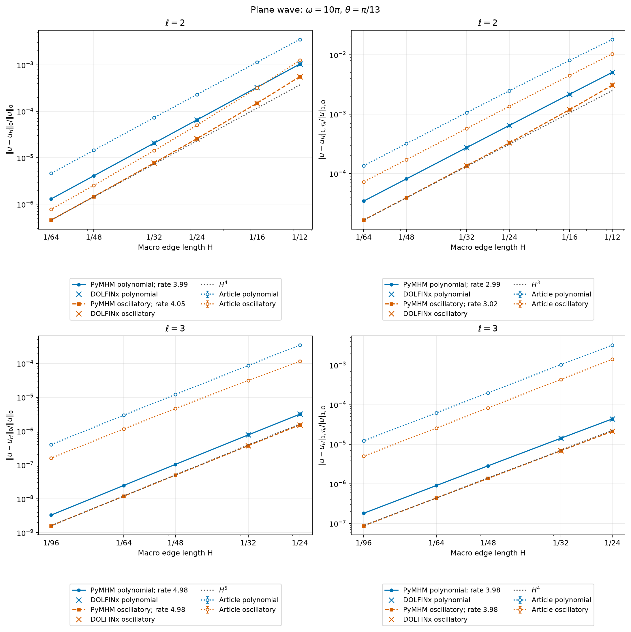
Face degree	Basis	Finest n	Relative pressure L2	Relative gradient L2
2	Polynomial	64	1.30047e-6	3.44183e-5
2	Oscillatory	64	4.56319e-7	1.64739e-5
3	Polynomial	96	3.30054e-9	1.80717e-7
3	Oscillatory	96	1.59577e-9	8.74003e-8

The plots include all 44 published markers, extracted from the PDF's vector paths with independently calibrated logarithmic axes. The declared coordinate interval gives at most 0.283% graphical uncertainty. The final published-to-computed error ratios are 3.55/1.70 for pressure and 3.93/4.40 for the gradient at \(\ell=2\) (polynomial/oscillatory). At \(\ell=3\) they are 120.6/99.8 and 67.6/57.1, respectively. Thus the asymptotic orders agree, but the error amplitudes do not. The unspecified historical finite local spaces prevent treating these results as a quantitative reproduction of Figures 6.6–6.7. The extracted values and their intervals retain the original coordinates and the corresponding PyMHM records.

The angular study contains 256 directions for each configuration and basis, as in Section 6.2: \((\ell,\omega,H)=(2,20\pi,1/11)\) and \((4,40\pi,1/21)\). The two bases have identical numbers of skeletal degrees of freedom within each comparison.

The polynomial gradient-error maxima are 0.157928 and 0.00521541 for \(\ell=2\) and \(\ell=4\), respectively. These values do not quantitatively match the approximately 0.021 and 0.022 peaks printed in Figure 6.5. The printed local discretization is unavailable; the discrepancy is not resolved by the following \(r=2,4,8\) local-resolution controls. Accordingly, these are verified calculations with the stated inputs, not a completed reproduction of the printed error ordinates.

At \(\theta=\pi/13\), the relative gradient errors are:

Trace degree	Basis	\(r=2\)	\(r=4\)	\(r=8\)
2	Polynomial	0.0538611	0.0539237	0.0539349
2	Oscillatory	0.0626927	0.0628351	0.0628407
4	Polynomial	0.00400911	0.00401787	0.00401881
4	Oscillatory	0.00101542	0.000995336	0.000995704

Here only the local subdivision changes. The macro mesh, trace space, frequency and source remain fixed. The small \(r=4\) to \(r=8\) increments show that further local refinement does not remove the observed discrepancy with the published amplitudes at this direction.

At the coordinate directions, the exact normal trace belongs to both skeletal spaces. The remaining error is the finite local approximation error: for \(\ell=2\), it falls from 0.0124188 to 0.000808348 on changing \(r=2\) to \(r=4\); for \(\ell=4\), it falls from 0.000279193 to 0.000004593. Directions between the exact ones can retain a skeletal error. An oscillatory basis is not uniformly more accurate at every propagation angle.

An independent DOLFINx 0.9.0/UFL application checks twelve complete hybrid systems: both published \((\ell,\omega,H)\) configurations, both trace families, and \(\theta=0,\pi/13,\pi/4\). It assembles the volume, impedance, incident-wave load and oriented face coupling independently, then solves the full complex saddle matrix with SciPy SuperLU, without condensation. Its polynomial and trigonometric trace coordinates and Cartesian face numbering are independent of PyMHM's coordinates. The larger systems contain 78,729 complex unknowns. The maximum difference between physical pressure coefficients is \(5.02\times10^{-11}\); independently integrated relative pressure and gradient errors differ by at most \(7.80\times10^{-13}\) and \(2.46\times10^{-13}\). The native verification record identifies versions, source digests, all twelve configurations and the original equation residuals. These checks verify the stated finite discretization; they do not identify the unknown historical discretization or remove the published-curve discrepancies above.

A second DOLFINx/UFL comparison uses the convergence problem itself: \(\omega=10\pi\), \(\theta=\pi/13\), two local subdivisions and Q\(_{\ell+2}\) fields. It checks both trace families at \(n=12,16,24,32\) for \(\ell=2\) and at \(n=24,32\) for \(\ell=3\). The largest uncondensed system has 131,840 complex unknowns. The independently integrated relative pressure and gradient errors differ from PyMHM by at most \(9.17\times10^{-14}\) and \(1.05\times10^{-14}\), respectively. On the final refinement interval, the independent pressure/gradient orders are 3.991/2.991 (polynomial) and 4.186/3.094 (oscillatory) for \(\ell=2\); for \(\ell=3\) they are 4.909/3.923 and 4.898/3.924. These agree with the expected asymptotic orders \(\ell+2\) and \(\ell+1\) for this smooth solution. The records identify the verified DOLFINx 0.9.0 release, its installed build and the separately written full-system assembly.

The separate outgoing-Hankel and PML studies retain their explicitly stated analytical data and grids. Their fields below use common physical scales.

All pressure and gradient norms use complex absolute squares at physical quadrature points. The displayed weighted error is

\[ \frac{ \bigl(\|\nabla(u-u_h)\|_{0,\mathcal T_H}^2 +\omega^2\|u-u_h\|_{0,\Omega}^2\bigr)^{1/2}} {\bigl(\|\nabla u\|_{0,\Omega}^2 +\omega^2\|u\|_{0,\Omega}^2\bigr)^{1/2}}. \]

Assembly uses ten Gauss points per coordinate and error integration uses twelve. Real and imaginary components retain their signs. Each analytical, numerical and error map shows the actual macro mesh and preserves independent local samples on its interfaces.

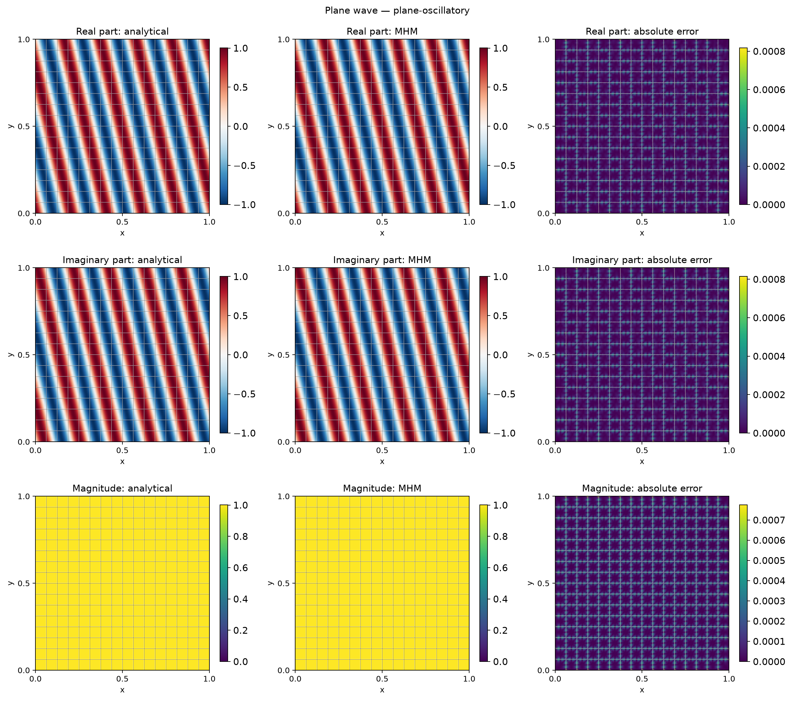
The spatial-map record identifies this \(n=16\), \(\ell=2\), local-Q4 case and its executed basis. Physical pressure and gradient norms agree with the retained configuration within \(2\times10^{-11}\) relatively; the reconstructed original local equations have relative residual below \(2\times10^{-16}\). The convergence-figure record separately identifies the literal measurements and source identities used in the convergence plot.

Pollution and the exact-flux interpolant

Section 6.1 separates the error of the MHM solution from that of the local lifting of the projected analytical normal flux. For the outgoing Hankel solution, define

\[ \begin{aligned} \lambda&=-\nabla u\cdot n,\\ u_{\mathrm{INT}}&=T(\Pi_H\lambda)+\widetilde T(g),\\ E_{\mathrm{MHM}}&=\|\nabla(u-u_H)\|_{0,\mathcal T_H},\\ E_{\mathrm{INT}}&=\|\nabla(u-u_{\mathrm{INT}})\|_{0,\mathcal T_H}. \end{aligned} \]

The projection is the facewise L2 projection in the oriented trace basis. Absorbing faces contribute through the original impedance load. The interpolant uses the same finite local inverse as the computed MHM field; it is neither a best approximation nor a separate global solve.

The four frequency/degree pairs are \((\ell,f)=(0,10),(0,20),(1,15),(1,75)\), where \(\omega=2\pi f\). Local Q\(_{\ell+3}\) fields use two subdivisions per macro direction; these finite local spaces are selected explicitly because the article does not specify them. Assembly, error integration and face projection use 12, 16 and 24 Gauss points per coordinate, respectively.

For the highest-frequency pair \((\ell,f)=(1,75)\), an independent DOLFINx/UFL full-system comparison uses the same Q4 local space, two local subdivisions and analytical impedance data on every exterior face. At \(n=16,32,64\), relative differences in pressure and its broken gradient are below \(9.4\times10^{-10}\), \(6.0\times10^{-14}\) and \(9.2\times10^{-13}\), respectively. The \(n=64\) system contains 347,904 complex unknowns. The native assembly uses an independent 24-point integration of the nonpolynomial boundary load; both the finite local spaces and that quadrature convention are recorded. This verifies the selected discrete Hankel problem, independently of whether its unspecified historical local spaces coincide with those of the article.

The sampled threshold is the largest recorded edge length for which \(E_{\mathrm{MHM}}\leq3E_{\mathrm{INT}}\) holds at every finer attempted resolution. Rejected local inverses interrupt this suffix. For example, \(\omega=30\pi\) and square edge \(H=1/30\) place an interior Neumann problem at its first continuous eigenfrequency. That grid is not an admissible intermediate point in a verified suffix. Neither a finite sampled suffix nor a nonsingular discrete matrix proves the condition at all unsampled mesh sizes.

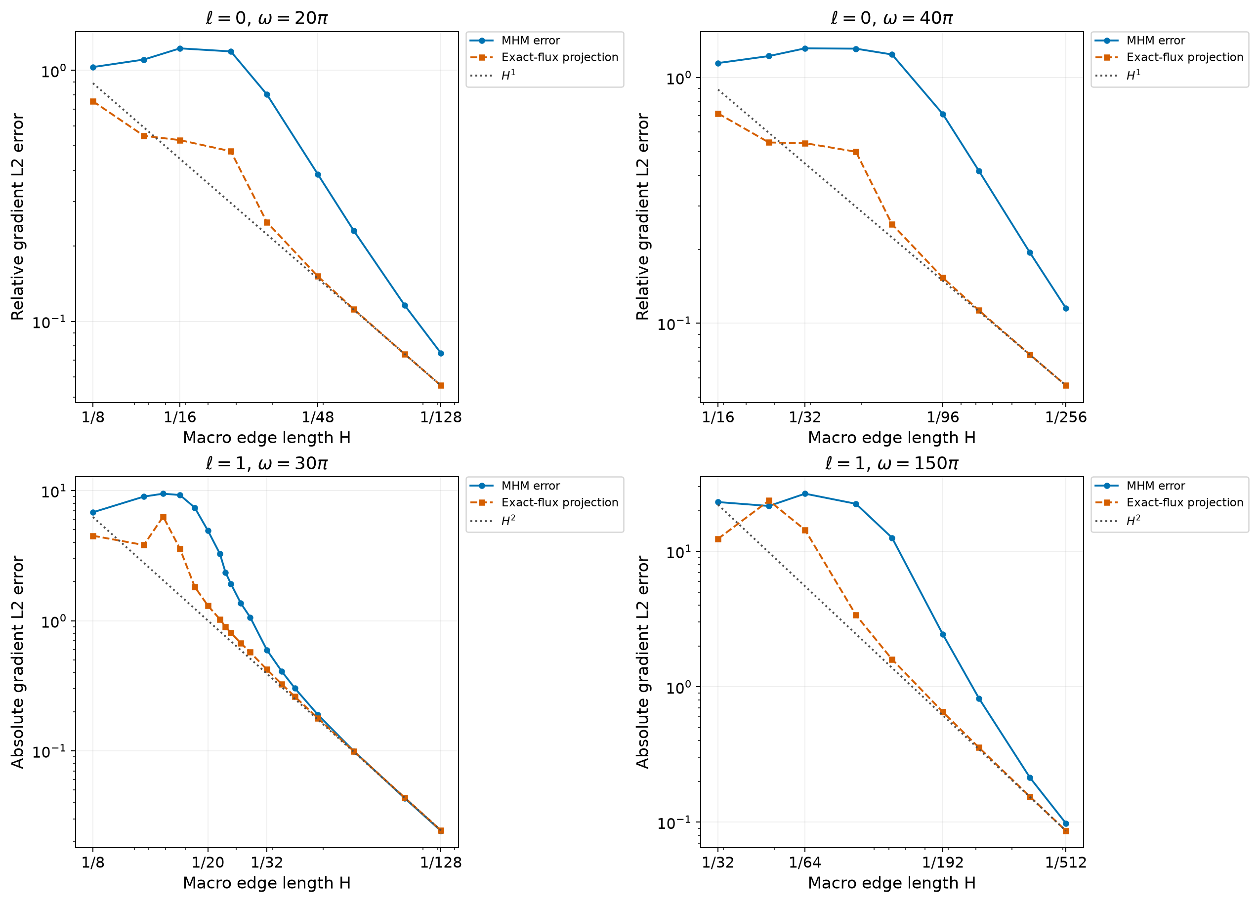
The refined sequences resolve the transition from pollution-dominated errors to ratios approaching one. The following thresholds concern the attempted admissible sequence, with the stated finite local spaces; they are not continuous bounds on all possible macro meshes.

Trace degree \(\ell\)	Frequency \(f\)	Attempted admissible grids	Finest \(n\)	Sampled suffix threshold \(H\)	Finest error ratio
0	10	9	128	\(1/48\)	1.35
0	20	9	256	\(1/192\)	2.06
1	15	18	128	\(1/32\)	0.992
1	75	9	512	\(1/256\)	1.134

At \((\ell,f)=(1,75)\) and \(n=512\), the absolute broken-gradient errors are \(0.09786\) for MHM and \(0.08630\) for the exact-flux interpolant. The finer \(n=256,384,512\) grids all satisfy the factor-three criterion. For \(f=15\), the rejected \(n=30\) local inverse separates the sampled admissible suffix from the coarser grids, even when a coarser error ratio is below three. The sequence records preserve every sampled value and its executed acquisition provenance.

Diagonal PML coordinates

Section 3.3 supplies the coordinate-transformed variant. For stretches \(s_x,s_y\) with positive real and nonnegative imaginary parts, the implementation uses

\[ D=\operatorname{diag}(s_y/s_x,s_x/s_y),\qquad d=s_xs_y, \qquad -\nabla\cdot(\rho^{-1}D\nabla u)-\omega^2\kappa^{-1}du=f. \]

pml_stretch is opt-in and requires absorbing=None. Dirichlet or transformed conormal data can be prescribed on the exterior. The source is the right-hand side of this transformed equation. Combining it with an untransformed impedance condition is not part of this API.

An original manufactured verification chooses \(\omega=10\pi\), \(s_y=1\) and

\[ \begin{aligned} s_x(x)&=1+\frac{150i}{\omega}(x-0.6)_+^2,\\ u(x,y)&=\exp\!\left(i\omega x-50(x-0.6)_+^3\right). \end{aligned} \]

This field has zero transformed source and analytical Dirichlet data. The study uses local Q4 and constant face traces. Its five main grids have \(n=16,20,24,28,32\), satisfying \(\omega H_K<\pi\) in the undamped region. These norms measure discretization error for this stated transformed problem; they do not measure an unbounded-domain PML truncation error.

The profile at \(y=0.473\) evaluates the archived Q4 polynomials on the \(n=24\) macro mesh, with independent incident values at fine and macro interfaces. Vertical lines mark that field's actual macro intersections.

Verification and use

The portable tests cover complex quadratic solutions under absorbing, Dirichlet, Neumann and mixed boundary conditions; independent uncondensed complex algebra; physical macro balances; planar and Cartesian material integration; local resonance rejection; and portable process assembly. Eight native DOLFINx/UFL comparisons verify P1/P3 and Q1/Q3 local matrices and loads, with and without complex PML coefficients. The PML and Hankel analytical data are also checked independently by differentiation.

pixi run --locked -e notebooks python -m examples.helmholtz_campaign --workers 8
pixi run --locked -e notebooks python -m examples.plot_helmholtz

The numerical records declare the executed spaces, physical norms and source digests. Notebook 61_helmholtz.ipynb provides a small complex patch and displays these records. The heterogeneous Marmousi experiment in Section 6.4 is not reproduced by these analytical-wave studies: its historical material preprocessing, point source, reference grid and sampled error definition require a separate matched data acquisition.

Marmousi II: published experiment and material identification

Section 6.4 and Table 6.1 of the Chaumont-Frelet and Valentin (2019) specify a \(10{,}240\,\mathrm{m}\times2{,}560\,\mathrm{m}\) domain, material arrays on a \(2048\times512\) Cartesian grid, \(\kappa=\rho c_p^2\), and a frequency of \(20\,\mathrm{Hz}\), so \(\omega=40\pi\,\mathrm{s}^{-1}\). The unit point source acts as \(v\mapsto v(5000,50)\). The top boundary is Dirichlet; the other three sides use the first-order absorbing condition. The published reference uses continuous triangular P4 elements, with two triangles in each square of the \(2048\times512\) material grid.

The MHM configurations are explicit:

Macro side \(H\) (m)	Cartesian macro grid	Local element	Local grid in each macrocell	Local cell side (m)
20	\(512\times128\)	Q3	\(8\times8\)	2.5
40	\(256\times64\)	Q3	\(16\times16\)	2.5
80	\(128\times32\)	Q3	\(32\times32\)	2.5

Table 6.1 measures pressure on a \(513\times129\) sampling grid. Its quantity is

\[ E_{\mathrm{sample}}= \left( \frac{\sum_{i=1}^{513}\sum_{j=1}^{129} \left\lvert u_{\mathrm{ref}}(x_i,z_j)-u_H(x_i,z_j)\right\rvert^2} {\sum_{i=1}^{513}\sum_{j=1}^{129} \left\lvert u_{\mathrm{ref}}(x_i,z_j)\right\rvert^2} \right)^{1/2}. \]

This sampled relative error is distinct from a quadrature-integrated physical L2 norm. The printed MHM values below are published percentages, not PyMHM results.

\(H\) (m)	\(\ell=0\)	\(\ell=1\)	\(\ell=2\)	\(\ell=3\)	\(\ell=4\)
20	138	2.90	0.13	0.11	0.03
40	225	45.1	1.47	0.37	0.20
80	161	154	44.8	4.12	0.33

The public Marmousi II dataset description identifies the velocity and density SEG-Y files. The examined files contain \(13601\times2801\) samples. Their native values use km/s and g/cm³, respectively; conversion to m/s and kg/m³ multiplies each by 1000. The image comparison uses nominal 1.25 m spacing over a \(17\,\mathrm{km}\times3.5\,\mathrm{km}\) domain. The archive's processing example instead writes 1.249 m; that convention is recorded separately and cannot be distinguished from these article rasters.

The material-identification record contains the primary download URLs, SHA-256 digests, image dimensions, all 270 fixed-size crop candidates and four correlations per candidate. The search retains the stated \(10.24\,\mathrm{km}\times2.56\,\mathrm{km}\) dimensions and varies only the crop origin in 5 m steps. At its best origin \((3395,515)\) m, the pattern correlations are:

Native field	Figure 6.8, titled velocity	Figure 6.9, titled density
P-wave velocity	0.780816	0.992889
Density	0.983439	0.784447

The stronger crossed association concerns the displayed patterns. It does not establish an interchange of density and velocity in the historical numerical operator. The horizontally symmetric crop beginning at \((3380,520)\) m also has high crossed correlations, 0.989650 and 0.980906. One image pixel spans approximately 20.65 m horizontally and 23.27 m vertically under the stated computational dimensions; the 15 m horizontal separation of these candidates is smaller than one pixel. These are image-localization scales, not statistical confidence intervals. The printed coordinate ticks suggest approximately \(9\,\mathrm{km}\times2\,\mathrm{km}\), adding a distinction between the displayed axes and the computational dimensions stated in the text.

Thus the images support an approximate central subfield, while the historical \(2048\times512\) coefficient arrays remain unidentified. Literal reproduction of Table 6.1 requires those arrays, their crop/resampling and cell-versus-node conventions, and the sampling rule on macro interfaces. The point source, boundary conditions, local Q3 spaces and classical P4 reference must also be matched. No material coefficient has been adjusted to reproduce the images, and this geometric evidence is not a numerical reproduction of Table 6.1.

The Marmousi point-source case specifies the selected coefficient arrays, executes independent classical refinements and compares their complex pressure and physical flux. It uses the published operator and numerical spaces while keeping the unresolved historical data conventions explicit.

References

• Théophile Chaumont-Frelet, and Frédéric Valentin (2020). A Multiscale Hybrid-Mixed Method for the Helmholtz Equation in Heterogeneous Domains. SIAM Journal on Numerical Analysis 58(2) 1029-1067. DOI: 10.1137/19M1255616.

• Théophile Chaumont-Frelet and Frédéric Valentin (2019). A multiscale hybrid-mixed method for the Helmholtz equation in heterogeneous domains. HAL author manuscript, version 2, submitted 16 April 2019. HAL: hal-01698914v2. The journal publication is SIAM Journal on Numerical Analysis 58(2), 1029–1067 (2020), DOI: 10.1137/19M1255616.