Conforming potential and an energy-error estimator

The scalar estimator in pymhm.estimators.darcy implements the unit-diffusion case of Section 5 in Barrenechea et al. (2026). It combines the RT moment reconstruction with a continuous recovered potential. The original broken MHM solution is preserved. This implementation assumes identity diffusion, homogeneous Dirichlet data, convex triangular macrocells and a globally conforming union of the fine meshes.

Four separately measured contributions

Write \(p_h\) for the primal MHM field, \(q_h\) for its recovered RT flux and \(I_{\mathrm{OS}}p_h\) for the Oswald potential. At an interior Lagrange node,

\[ (I_{\mathrm{OS}}p_h)(z)=\frac{1}{\#\mathcal T_z} \sum_{T\in\mathcal T_z}p_h|_T(z). \]

The average counts incident fine triangles, including repeated values from one macrocell. Boundary nodes are set to zero. For a uniform polynomial degree and matching fine edges this defines a continuous finite-element function in \(H^1_0(\Omega)\). The recovered potential and the original broken field are displayed as separate mathematical quantities.

Let \(\Pi_{K,m}\) denote the L2 projection onto continuous piecewise Pm functions on the fine triangulation of macrocell \(K\). It is not the discontinuous cellwise projection. With \(H_K=\operatorname{diam}(K)\), the four terms are

\[ \begin{aligned} \eta_{1,K}&=\|\nabla p_h+q_h\|_{0,K},\\ \eta_{2,K}&=\|\nabla(p_h-I_{\mathrm{OS}}p_h)\|_{0,K},\\ \eta_{3,K}&=\frac{H_K}{\pi} \|\Pi_{K,m}(\operatorname{div}q_h)-\operatorname{div}q_h\|_{0,K},\\ \eta_{\mathrm{osc},K}&=\frac{H_K}{\pi}\|f-\Pi_{K,m}f\|_{0,K}. \end{aligned} \]

The full indicator is

\[ \eta^2=\sum_K(\eta_{1,K}+\eta_{3,K}+\eta_{\mathrm{osc},K})^2 +\sum_K\eta_{2,K}^2. \]

For the theorem's hypotheses and exact integration, \(\|\nabla(p-p_h)\|_{0,\mathcal P}\leq\eta\). The constant \(H_K/\pi\) uses convexity of each macrocell. The hypotheses include local degree \(k\geq\ell+2\) and \(\ell\leq m\leq k\), where \(\ell\) is the skeletal degree. The implementation accepts general nonnegative RT orders \(m\) subject to these space conditions and adequate quadrature. The five-level campaigns below use RT2 reconstruction; their numerical evidence does not extend automatically to every supported order.

The cited analysis also uses independent polynomial tests on every skeletal subface. Its local efficiency proof tests a constant supported on one subface to obtain a zero mean pressure jump there. Continuous polynomials on a face with several segments remove those individual tests, so this estimator API rejects that choice. A continuous face with a single segment has the same polynomial space as its discontinuous counterpart. RT moment reconstruction remains available for subdivided continuous traces; that algebraic construction does not transfer the estimator's theorem to the reduced test space.

Neither an arbitrary SPD coefficient nor nonzero boundary data is accepted under this formula. In particular, a coefficient-dependent energy bound must not be inferred from the unweighted unit-diffusion flux norm. More general coefficient weights and boundary liftings require their own derivation.

API and numerical safeguards

The example helpers below are repository sources, supplied separately from the installed library. Open the corresponding notebook to acquire its verified companion, as described in the notebook guide.

from pymhm import TriangleMesh
from examples.formulations.application import darcy as solve_darcy
from pymhm.estimators.darcy import estimate_darcy_error

solution = solve_darcy(
    TriangleMesh.unit_square(4), degree=2,
    source=lambda x: x[:, 0], quadrature_order=8,
)
estimate = estimate_darcy_error(
    solution, homogeneous_dirichlet=True, degree=2, quadrature_order=10,
)
print(estimate.total)
print(estimate.local_squared)

homogeneous_dirichlet=True is a required declaration: DarcySolution does not retain its original boundary specification. The estimator additionally checks the computed zero Dirichlet moments on exterior macrofaces; it does not demand pointwise zero boundary values from the broken MHM field. Nonmatching fine boundaries, incompatible local/trace degrees, nonidentity coefficients and failed continuous-test equilibrium are rejected.

equilibrium_defect records the source-minus-divergence moment defect on each macrocell. Estimator projections and norms use the requested quadrature, and energy_error(exact_gradient, order=...) uses independent error quadrature. The recovered flux stores its own quadrature order for subsequent projection diagnostics. Assembly and diagnostic quadratures control different errors: the source load remains determined by the assembly rule.

The theorem assumes exact integration. These outputs are floating-point, quadrature-based estimates, checked against analytical errors in the examples; they are not interval-certified bounds. The complete estimator includes source oscillation and the nonzero divergence-projection defect. Omitting either term would be a different estimator.

Five macro meshes

The analytical problem is the sine case from Section 6.1:

\[ p=\sin(2\pi x)\sin(2\pi y),\qquad f=8\pi^2p,\qquad q=-\nabla p. \]

The macro mesh has \(2n^2\) diagonal triangles for \(n=1,2,4,8,16\), each subdivided into four fine triangles. We compare \((\ell,k,m)=(0,2,2)\) and \((1,3,2)\). Assembly and estimator quadrature use Duffy order 10; independent energy and pressure errors use order 12. These are declared package calculations of the published analytical problem, not a claim of equality with the article's tables.

The projected-divergence and source-oscillation contributions differ from Table 3 for the declared meshes. Exact historical macro/fine connectivity and executable estimator/projection inputs are unavailable, so the cause of that discrepancy is unresolved.

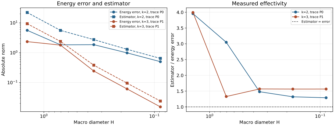
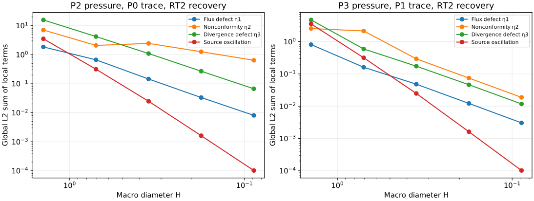
Effectivity is \(\eta/\|\nabla(p-p_h)\|\), using the actual broken gradient. A value above one is the expected upper-bound behavior. Coarse preasymptotic errors need not decrease monotonically. Component curves are norms of local terms, while the full estimator combines them by the formula above.

n	P2/P0 energy error	P2/P0 estimator	Effectivity	P3/P1 energy error	P3/P1 estimator	Effectivity
1	5.63376	22.2834	3.95533	2.34914	9.3771	3.99172
2	1.83747	5.59985	3.04758	1.80008	2.39124	1.32841
4	1.86087	2.75421	1.48006	0.24349	0.381949	1.56865
8	0.986555	1.30158	1.31932	0.0609796	0.0954082	1.56459
16	0.50101	0.646038	1.28947	0.0152811	0.0239186	1.56524

The largest continuous-test equilibrium moment norm in these ten runs is \(6.98\times10^{-14}\). Estimator quadrature refinement and a cubic exact triangle bubble are separate regression checks.

Original and recovered fields

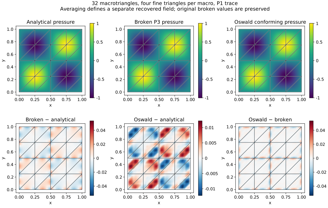
The displayed case has 32 macrotriangles, P3 primal pressure, P1 skeletal traces and RT2 recovery. The first row shares a color scale; the second row uses separate signed-error scales. Every panel overlays the actual macro mesh. The Oswald potential is continuous and has the prescribed zero boundary trace. This property alone does not guarantee that its L2 error is smaller for every problem.

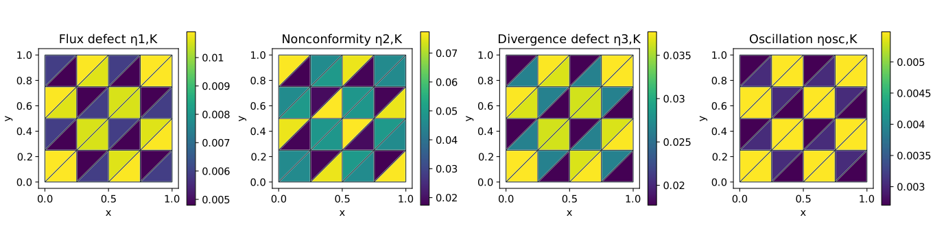
Each colored macrotriangle shows its integrated local norm, without dividing by its area. These indicators provide cellwise quantities for mesh marking. The example uses prescribed meshes and does not implement an adaptive refinement loop or establish contrast-uniform efficiency. The article's efficiency estimates contain mesh-ratio and additional flux/oscillation terms.

pixi run --locked -e notebooks python -m examples.plot_estimator
pixi run --locked -e notebooks python -m examples.plot_estimator --reuse-results

The first command solves and archives examples/results/estimator.json and sampled potential fields. The second redraws those records without solving. Notebook 20_darcy_estimator.ipynb runs a small consistency check and displays the preserved five-level figures.

References

• Gabriel R. Barrenechea, Larissa Martins, Weslley Pereira, and Frédéric Valentin (2026). An H(div; Ω)-Conforming Flux Reconstruction for the Multiscale Hybrid-Mixed Method, Multiscale Modeling & Simulation 24(2), 399–428. DOI: 10.1137/24M1673073.