Darcy-coupled transient transport

solve_transient_transport advances

\[ \rho\,\partial_t u-\nabla\!\cdot(D\nabla u) +\nabla\!\cdot(\beta u)+cu=f \]

with backward Euler, continuous local Pk fields, and the conservative hybrid Robin trace. Capacity is positive, and the spatial coefficients are stationary; sources and boundary data may depend on time. Both Galerkin and consistent SUPG testing include the time residual. In particular, the previous solution enters through the same weighted mass form as the current time derivative.

OfflineHybridSystem prepares local and global factors once per distinct time increment. Changes in sources and boundary values only rebuild loads. The reported operator_builds counts these prepared time-step operators; it is not a performance speedup measurement.

For long trajectories, output_steps selects the one-based step indices retained in the result. Every time step is computed; integration_times records the entire grid, while times, solutions and balance records refer to the selected outputs. The optional on_step(step, time, solution, balance) callback receives read-only numerical arrays after each computed step, including steps omitted from the returned history. This permits checkpointing without keeping every state in RAM. Callback exceptions close the prepared local and global factorizations.

With check_original=True, every time step also passes the shared verification of the original local equations, free weak trace equations and physical moments, with tolerance \(10^{-10}\) relative to the physical right-hand side. Prescribed trace values are moved to that right-hand side. This check leaves the executed solution unchanged and performs no correction. original_residual_norms and original_rhs_norms record all computed steps in integration_times[1:] order, including steps omitted from the retained field history. Algebraic satisfaction does not establish approximation accuracy or inf-sup stability.

Conservative Darcy velocity and dispersion

Section 5.4 of Harder, Paredes and Valentin (2015) couples a stationary Darcy field to transport with hydrodynamic dispersion. solve_darcy_transport accepts locally H(div)-conforming RT and BDM Darcy solutions, including RT moment reconstructions. It evaluates their actual physical vector polynomials without changing the Darcy approximation:

\[ \beta=q_h,\qquad D(q_h)=(\alpha_m+\alpha_t|q_h|)I+ (\alpha_l-\alpha_t)\frac{q_h\otimes q_h}{|q_h|}. \]

At zero flux the tensor equals \(\alpha_m I\). The coefficients satisfy \(\alpha_m>0\) and \(\alpha_l\ge\alpha_t\ge0\). Within a two-dimensional RT0 triangle, \(\nabla q_h=bI\), where \(b=\nabla\!\cdot q_h/2\), so its broken tensor divergence away from zero flux is

\[ \nabla\!\cdot D=(2\alpha_l-\alpha_t)b\frac{q_h}{|q_h|}. \]

This derivative is included in SUPG. At isolated zero-flux points the formula is understood almost everywhere; no derivative across a material interface is inserted into a fine-element residual.

The transport fine triangulation matches the Darcy fine triangulation. The coupling passes the actual Darcy partitions to every transport operator; matching cell counts alone is insufficient. An explicit mesh override must preserve their points and connectivity. Standalone heat and transient transport also accept validated local_meshes, which take precedence over uniform refinement and define both the old-state interpolation and the new-state forms. MacroCoefficient and RT0DarcyVelocity preserve the macro side when evaluating broken coefficients. A barycentric membership check validates each fine-cell location; nearest-centroid selection alone is insufficient. Raw primal Darcy gradients are not silently substituted for a conservative velocity.

With velocity_representation="primal", the coupling instead retains the raw Darcy volume vector \(q_h=-K\nabla p_h\) and the Darcy skeletal multiplier \(\lambda_D\) as numerical normal flux. It integrates the Galerkin advection form directly:

\[ a_{\mathrm{adv},K}(u,w) =-\int_K q_hu\cdot\nabla w +\frac12\int_{\partial K}\lambda_Duw. \]

This pair preserves separate volume and skeleton approximations. It is not asserted to be H(div)-conforming: replacing its interface distributions by a broken divergence would give a different operator. The material's broken tensor derivative must be supplied explicitly as permeability_gradient; use 0.0 for a piecewise constant field. Darcy and transport face partitions and degrees may differ. Strong-residual stabilization is supported for the H(div) path and is rejected for the primal volume/numerical-normal pair.

Exterior diffusive_flux data prescribe \((-D\nabla u)\cdot n\). This permits strong inflow concentration together with homogeneous diffusive outflow and wall conditions, as in the published transport configuration. The package also supports explicitly prescribed Robin data through neumann.

A selected heterogeneous realization

examples/transport_random_campaign.py declares the first heterogeneous configuration from Section 5.4 on the full domain: 512 macrotriangles, 64 fine P3 triangles per macro, Darcy P2 traces on two segments, and transport P2 traces on eight segments. It uses unit capacity, zero initial concentration and source, strong concentration one at the left boundary, and zero diffusive flux on the other exterior faces. Backward Euler uses a time increment of 0.001 up to time seven, with the dispersion parameters stated above.

The saved permeability array has 64 by 16 values. Its selected realization uses PCG64 seed 20261003 with independent base-ten logarithms uniform on [-2,1]. The selected Darcy drive prescribes pressure three and zero on the left and right sides, with zero normal flux on the horizontal sides. The article does not supply its array, probability law, seed or exterior Darcy drive; these declared inputs do not identify its historical realization. Acquisition reads the actual saved array rather than regenerating it from the seed.

pixi run --locked -e test-core python -m examples.transport_random_campaign

Each observed field retains its physical nodal coefficients, executed basis matrices and orientation maps. Interior transport multipliers use half the Darcy numerical normal velocity, natural exterior multipliers represent diffusive flux, and removed strong-inflow trace coefficients prescribe no physical flux. The initial archive is an interpolation. These archives replay observed fields; they do not restart the integrator. Every computed step records its original-equation checks and nodal extrema, including steps omitted from the field history. The Galerkin method does not enforce concentration positivity.

The verified acquisition and replay pilot uses 32 macrotriangles and five time steps on the same domain and saved material. An independent full assembly using Basix 0.9.0, modules basix.finite_element and basix.polynomials, agrees at the first and fifth steps within 7.44e-13 relative in concentration L2 and broken gradient norms. The interior Robin norm differs by at most 3.53e-12 relative; the natural diffusive multiplier is zero in both fields. Both executed bases are evaluated on the same physical norm points. Candidate fields inserted into the independent original augmented equations have relative residual at most 1.29e-13, with the physical mass/source and strong-data right-hand side. The native homogeneous constant-state control preserves concentration one within 1.21e-13 through five steps. The separate control with the archived heterogeneous Darcy field and initial concentration one preserves this state within 3.37e-12. This verifies the original macro weak coupling; it does not make the primal volume velocity an H(div) field. The reference is an independently instrumented adapter, separate from the article authors' application and from a refined continuum reference.

The complete 512-macro trajectory, quadrature and space/time controls, and independently refined conforming references remain pending. A classical RT0 velocity is a separate approximation from the declared primal Darcy volume and skeletal pair.

An independently assembled classical reference uses conforming RT0/P0 for Darcy and continuous P3 with consistent mass for conservative transport. The saved material, pressure drive, initial and boundary data, dispersion law and time step are identical to the selected problem. Five-step pilots cover the whole domain on 2048 and 8192 triangles. They retain the executed Basix bases, physical operators, normal orientations, portable coefficients and strong-boundary dual reactions. The checkpoint contract includes the executed backward-Euler matrix and predecessor coefficients; replay with one and two native threads is identical without a fresh field solve. Native tests independently verify polynomial fields, RT normal integrals, the physical gauge, constant-state conservation and positive-quadrature norms.

At time 0.005, the 2048-to-8192-triangle increment is 36.15% in Darcy-flux L2 and 52.72% in concentration H1, using the finer computed norm as denominator. Same-space q8-to-q10 sensitivity is approximately 1e-15 in that pilot. These increments leave reference accuracy unresolved; the five steps do not establish a baseline for the full trajectory to time 7. Nodal undershoots are retained without clipping. The adapter executes Basix 0.9.0 at the verified project revision; its module is classical_reference.py, independently instrumented for this selected realization. The original classical application's source and 32000-triangle connectivity are unavailable.

The initial temporal control uses the same 2048-triangle spatial discretization with time steps 0.001, 0.0005 and 0.00025. At the common physical time 0.005, the concentration H1 increments are 0.5955% and 0.3141%, respectively, using the finer computed field as denominator. Positive q6/q8 integration gives the same norms, and all archived checkpoints replay identically with one and two native threads. These measurements concern one initial time; they do not establish a resolved full-trajectory reference or the convergence rate of a smooth analytical problem.

A five-level temporal verification

The recorded test is an original manufactured problem using the article's coupling and dispersion law. It does not reproduce the article's unspecified random permeability realization. On \([0,3]\times[0,1]\), set

\[ K(y)=\begin{cases}1,&y<1/2,\\10,&y\ge1/2,\end{cases}\qquad p=3-x,\qquad q=(K(y),0), \]

and

\[ \begin{aligned} u&=e^{-t}b(x),\qquad b(x)=1+\frac{x(3-x)}9,\\ f&=e^{-t}\left[-b(x)+\frac{2(\alpha_m+\alpha_lK)}9 +\frac{K(3-2x)}9\right]. \end{aligned} \]

The concentration is prescribed strongly on \(x=0,3\); the remaining exterior sides have zero diffusive flux. Initial data are \(b\). The layer interface aligns with the fine and macro meshes, and normal advective and diffusive fluxes across it are zero. The parameters are \(\alpha_m=10^{-6}\), \(\alpha_l=10^{-2}\), \(\alpha_t=10^{-3}\), unit capacity, and zero reaction.

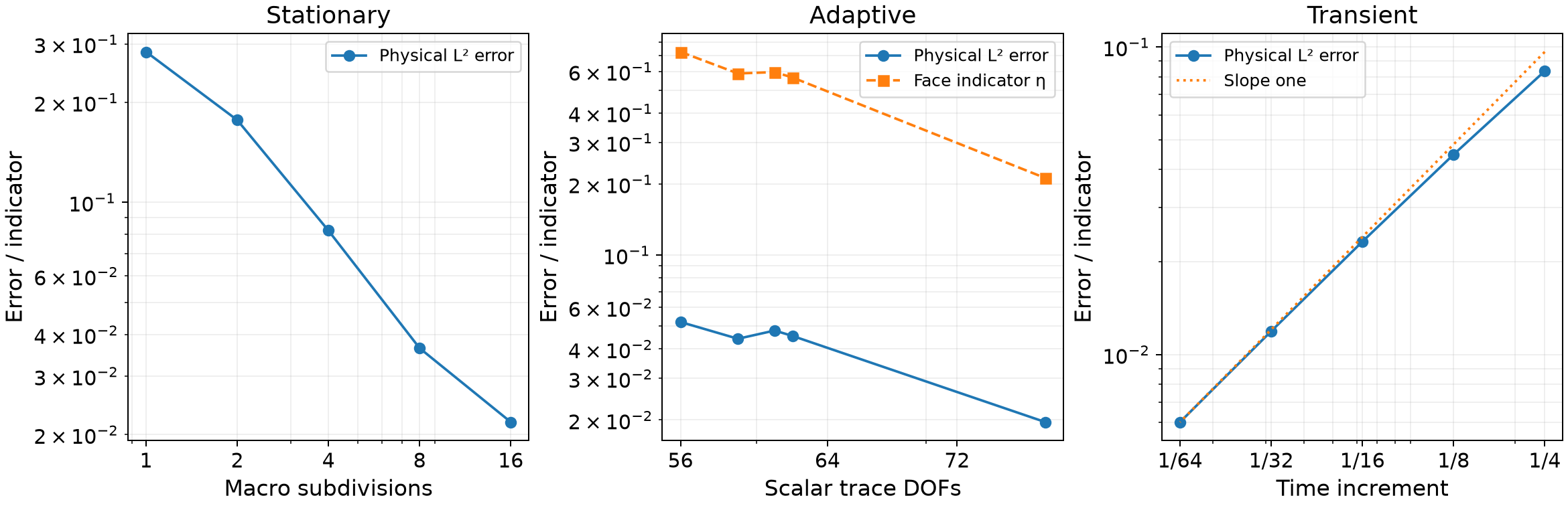
Darcy uses RT0/P0 on sixteen fine triangles per macrotriangle. Transport uses local P3 and degree-two macroface multipliers, with SUPG. Five uniform time grids contain 4, 8, 16, 32 and 64 steps up to \(t=1\). The exact concentration and independent error quadratures distinguish temporal truncation from algebraic residuals.

Steps	Time increment	L² error at t=1	Prepared operators
4	1/4	0.08350081	1
8	1/8	0.04469750	1
16	1/16	0.02328481	1
32	1/32	0.01190523	1
64	1/64	0.00602688	1

The last doubling gives an observed temporal order of 0.982. The computed Darcy flux has L² error \(4.79\times10^{-15}\) for this exactly representable field. The largest discrete balance residual is \(2.19\times10^{-14}\). Error quadratures of orders 10 and 12 differ by less than \(7\times10^{-17}\).

The current-source replay identifies the campaign and field archive by SHA-256 and reproduces all five temporal records and all seven saved field arrays bitwise. Its source hashes describe this replay, separately from the original acquisition. The same record documents the custom-partition regressions and independent UFL checks of the backward-Euler Galerkin and SUPG operators.

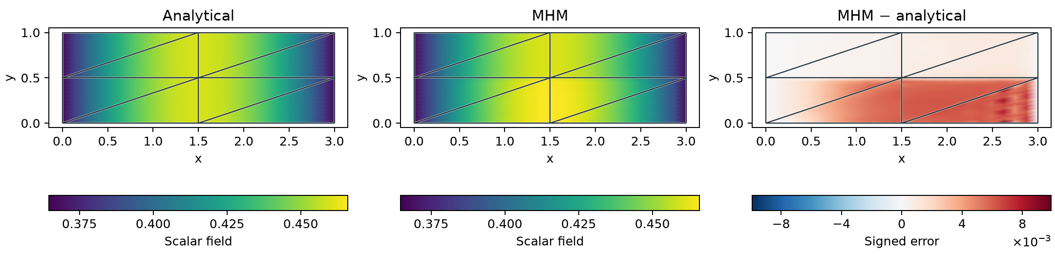
This map uses the eight-macrotriangle mesh of the five-level temporal test, with 64 time steps. The application Gallery uses 128 macrotriangles and includes separate temporal and spatial controls. Both retain the same layered Darcy operator and concentration data. The field-map record identifies this 64-step reconstruction; its independently integrated error agrees with the temporal record within \(5\times10^{-13}\) relatively.

total_mass() integrates \(\rho u_h\) using the capacity-weighted mass moments. balance_residuals sums the original local scalar equations, including reaction forces from strongly imposed data. It is a discrete weak balance diagnostic; it is not a claim of fine-element conservation, an independent physical error, or a positivity certificate.

The source is available as examples/transport_campaign.py. Run pixi run --locked -e notebooks python -m examples.transport_campaign --collect to recompute all levels, or omit --collect to render the archived results. The lightweight test suite separately checks a linear-in-time variable-coefficient patch, mass preservation with closed boundaries, the heat limit, exact RT0 evaluation, and the dispersion derivative.

References

• Christopher Harder, Diego Paredes, and Frédéric Valentin (2015). On a Multiscale Hybrid-Mixed Method for Advective-Reactive Dominated Problems with Heterogeneous Coefficients, Multiscale Modeling & Simulation 13(2), 491–518. DOI: 10.1137/130938499.