Stokes–Brinkman estimation and adaptive meshes
This case evaluates the two-level estimator and both refinement strategies of Araya, Rebolledo and Valentin (2021) for the Stokes–Brinkman problem. The local formulation uses the velocity-gradient viscous operator, continuous equal-order velocity and pressure, and residual stabilization. The first and second levels of the estimator are recorded separately; their sum is not asserted to be a numerical upper bound with constant one.
Estimator and two distinct marking rules
For a macroface \(F\), split into segments \(\widetilde F\), define
The denominator is the original macroface length. Interior faces appear in both adjacent macrocell boundary sums. The second level contains fine-cell momentum residuals, divergence, and complete pseudotraction jumps or mismatch with the skeletal field. The residual stress is \(t_h=(\nu\nabla u_h-p_hI)n\), whereas the skeletal multiplier is \(\lambda=(-\nu\nabla u+pI)n\). The boundary mismatch is consequently \(t_h+\lambda_h\), with the incident orientation applied to \(\lambda_h\). Unlike the Oseen estimator, the Stokes–Brinkman estimator has no factor \(2^{-2\ell}\):
adapt_flow_macros implements Algorithm 1. It computes
\(\eta_K=\eta_{2,K}+\sum_{F\subset\partial K}\eta_{1,F}\), marks
\(\eta_K\geq\theta\max_T\eta_T\), and refines the selected macrotriangles.
Conforming red–green closure is explicit. Each child retains its parent's local
subdivision count: no independent local refinement accompanies this step.
The optional macro_refiner="longest-edge" uses conforming longest-edge
propagation with the same indicator and inherited local resolution. This
choice controls shape deterioration during repeated local marking; numerical
records identify the closure and the minimum macro angle.
adapt_flow(..., estimator_variant="stokes-brinkman-2021") implements
Algorithm 2. Its face indicator is
\(\eta_F=\eta_{1,F}+\sum_{K\in\omega_F}\eta_{2,K}\). It marks faces above
\(\theta\max_E\eta_E\), then bisects only the segment or tied segments
attaining the maximum first-level indicator within each marked face.
If \(\eta_{1,F}<\sum_{K\in\omega_F}\eta_{2,K}\), every adjacent local mesh
is also refined. Uniform rational-grid closure resolves all new trace
breakpoints. This closure, the threshold and the stopping limit are declared
parameters; the paper does not specify its historical mesh connectivity.
An alternative local_refiner="longest-edge" closes each new trace vertex
by refining only the necessary local boundary triangles and their conforming
neighbors. By default, local-error dominance refines all triangles of the
selected local mesh once. With local_error_marking="maximum", the fine-cell
contributions to \(\eta_{2,K}^2\) instead select cells whose contribution norm
is at least \(\theta\) times its local maximum. An interior fine-face residual
is split equally between its two adjacent cells; their sum preserves the
published local indicator. Every triggered local mesh is refined. The paper by Araya, Rebolledo and Valentin (2021) does
not prescribe this within-local selection, which is an explicit implementation
choice. This avoids imposing a uniform grid throughout a macrocell
solely to resolve a small boundary segment. The actual local meshes replace
uniform subdivision counts, and max_local_cells supplies an explicit cap.
Both APIs require full Dirichlet data for this estimator. They preserve the original linear-system tolerances and expose a separate stop reason when a requested resolution exceeds the configured memory cap.
solve_flow and solve_brinkman also accept local_meshes, an explicit tuple
of conforming triangular partitions, one per macrocell. Each partition must
cover its macrocell; the adaptive closure additionally resolves new skeletal
breakpoints. Supplying these meshes replaces uniform local_refinement;
the returned solution retains the
actual local meshes for evaluation, residual integration and visualization.
local_refiner controls their adaptive closure, while macro_refiner controls
the distinct operation of changing the macro partition.
Polynomial problem and viscosity
On the unit square, the campaign uses
with \(f=-\nu\Delta u+\nabla p\), zero velocity boundary data, and zero mean pressure. Here the symbol \(\nu\) denotes viscosity; the vector field in the display is \(u\). The two viscosities are 1 and \(10^{-2}\). Derivatives and forces are computed analytically from the polynomial.
The printed component ordering in §5.3 is not solenoidal. This experiment states the divergence-free streamfunction convention explicitly. Consequently, it is a verification with the published pressure, amplitudes and approximation families, rather than an assertion that an incompatible printed component pair solves the incompressible equations.
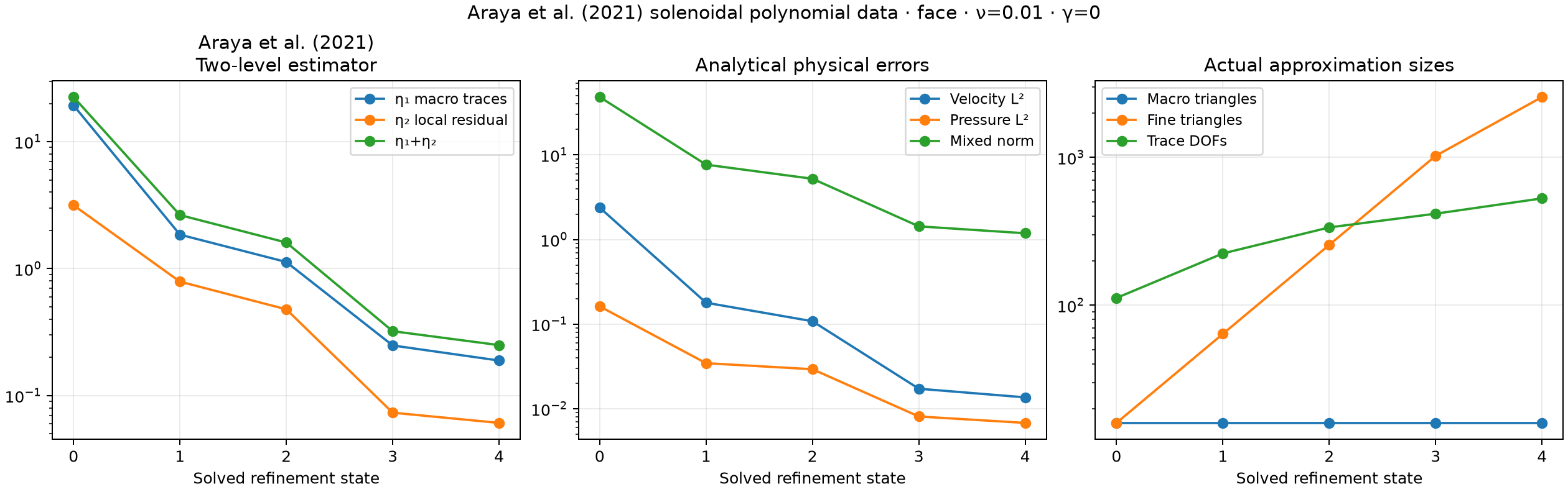
Six uniform series use local P3/P3, skeletal degrees 0, 1 and 2, and \(H=1/2,1/4,1/8,1/16,1/32\). Each macrotriangle contains one local triangle. The macro grid is a declared structured crisscross mesh. The physical velocity and pressure L2 errors and the paper's mixed norm are integrated independently of the discrete residual. Adaptive experiments use \(\theta=0.5\), four refinement steps, and keep the two marking strategies separate.
The effectivity reported here is always \((\eta_1+\eta_2)/\text{error}\). The preprint's Tables 1–2 contain entries whose printed effectivity instead matches \(\eta_1/\text{error}\), while Tables 3–4 contain sum-based entries. That printed column is therefore not a universal numerical equality check. The individual errors and estimator components remain the quantities used for comparison.
At \(H=1/32\), the measured mixed errors and effectivities are:
| Viscosity | Trace degree | Mixed error | η / mixed error |
|---|---|---|---|
| 1 | 0 | 0.568624 | 0.8280 |
| 1 | 1 | 0.00528972 | 4.2709 |
| 1 | 2 | 0.000163361 | 16.5335 |
| 0.01 | 0 | 39.1393 | 0.5613 |
| 0.01 | 1 | 0.192249 | 0.4600 |
| 0.01 | 2 | 0.000125147 | 0.3722 |
The curves resolve approximation order and viscosity sensitivity, but do not coincide in every component with the printed tables. The solenoidal component convention, declared mesh and computable polynomial inverse constant are part of this experiment's specification. Identical historical inputs are not established, and no estimator factor is adjusted to fit the tabulated values. Effectivity below one is compatible with an estimate having an unspecified reliability constant; it is not a guaranteed unit-constant upper bound.
The two adaptive campaigns start from different trace spaces: Algorithm 1 uses P0 and Algorithm 2 uses P1 for this polynomial test. Their work counts and accuracy therefore describe separate configurations, rather than an efficiency ranking of the marking rules. After four refinement steps:
| Viscosity | Strategy | Macro / fine triangles | Velocity L2 error | Pressure L2 error | Mixed error |
|---|---|---|---|---|---|
| 1 | Macro, P0 trace | 1,124 / 1,124 | 0.0199278 | 0.636720 | 1.21186 |
| 1 | Face, P1 trace | 16 / 4,096 | 0.000909202 | 0.0448634 | 0.0760168 |
| 0.01 | Macro, P0 trace | 1,832 / 1,832 | 1.38933 | 0.469148 | 73.1837 |
| 0.01 | Face, P1 trace | 16 / 2,560 | 0.0136072 | 0.00679364 | 1.18485 |
Regularized cavity and independent classical reference
The cavity uses \(ν=1\), \(γ=0\) or \(10^4 I\), zero volume force and zero mean pressure. On the top wall its velocity is \((16x^2(1-x)^2,0)\); the other walls are stationary. This continuous corner-compatible lid is a declared variation of the cavity in §5.4, whose corner convention and adaptive threshold are not specified. It is not presented as an identical reconstruction of Figures 2–3. Both adaptive strategies use local P2/P2 and P0 traces in this test.
The independently assembled conforming P2/P1 reference uses DOLFINx 0.9.0 and PETSc/MUMPS on seven nested grids, from \(8\times8\) through \(512\times512\) squares, each split into two triangles. The final system has 2,364,419 unknowns. The residual includes every pressure equation after the zero-mean gauge is restored. The reference's own last refinement differences are separate from the MHM differences:
| Drag | Relative velocity L2 change | Relative pressure L2 change | Relative velocity H1 seminorm change |
|---|---|---|---|
| 0 | 0.0000260% | 0.002027% | 0.005415% |
| 10,000 | 0.03491% | 0.002316% | 0.5481% |
Comparison norms integrate over every actual MHM fine triangle, including independent values at macro interfaces. Gaussian orders 12, 20 and 28 check intersections with the continuous reference. The maximum order-20 to order-28 change in the relative energy difference is 0.00060 percentage point. For \(e=u_h-u_{\rm ref}\), the velocity energy norm here is \(\big(\|\nabla e\|^2+\gamma\|e\|^2\big)^{1/2}\). After four adaptive steps, the differences relative to the corresponding reference norm are:
| Drag | Strategy | Macro / fine triangles | Velocity L2 | Pressure L2 | Velocity energy |
|---|---|---|---|---|---|
| 0 | Macro | 570 / 570 | 5.904% | 8.996% | 18.692% |
| 0 | Face/local | 16 / 808 | 13.272% | 19.071% | 25.846% |
| 10,000 | Macro | 146 / 146 | 28.000% | 70.231% | 30.688% |
| 10,000 | Face/local | 16 / 1,576 | 17.378% | 45.150% | 15.856% |
For the high-drag reference, its last relative energy increment is about 0.395%, well below the smallest MHM energy difference in the table. This distinguishes reference sensitivity from the remaining coarse-trace and local approximation error; it does not make the numerical reference exact. Neither the estimator nor its divergence component decreases monotonically in every adaptive sequence. Four steps are a finite verification campaign, not an assertion that the chosen meshes have reached a prescribed accuracy.
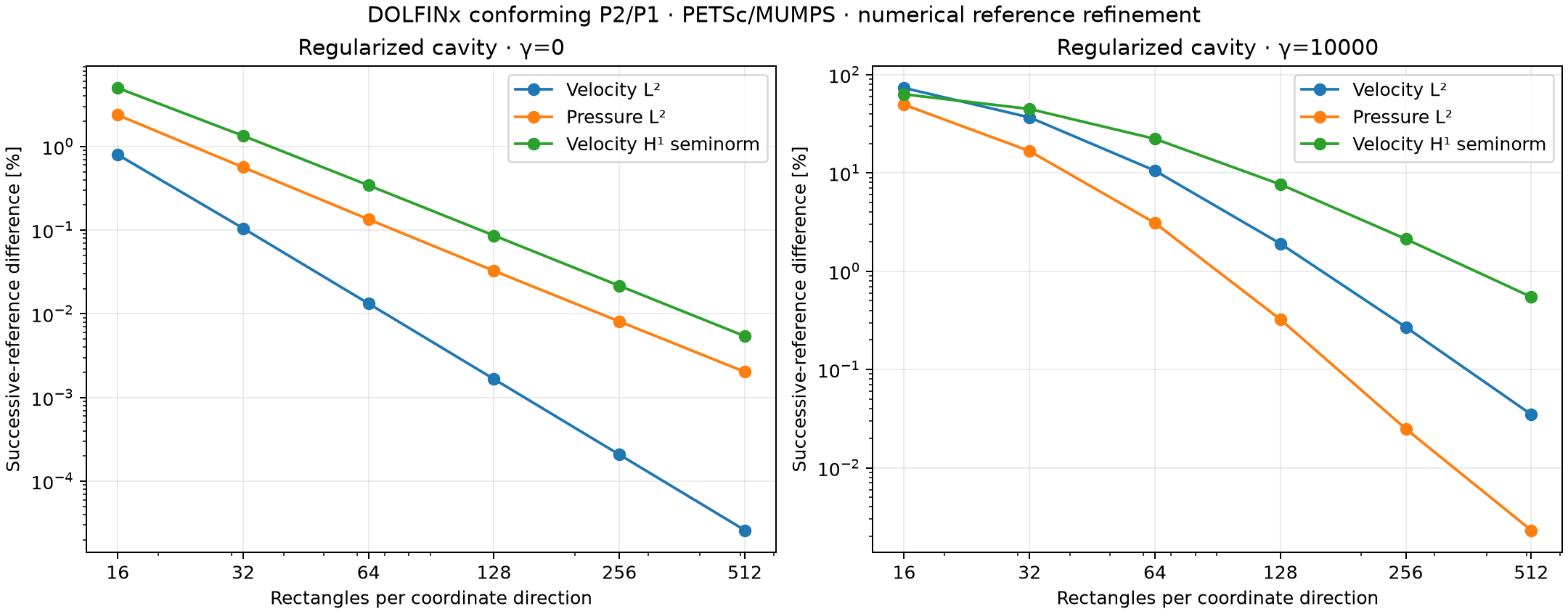
The plot uses the independently assembled reference's recorded refinement increments. Spatial maps comparing MHM with the \(512\times512\) reference require the separate original coefficient arrays; they are not inferred from these integrated differences.
Constant lid and corner singularities
The separate constant-lid case uses \(u=(1,0)\) on the open top edge and zero velocity on the other open edges, as in the cavity model of Araya, Rebolledo and Valentin (2021), §5.4. The MHM boundary functional integrates that discontinuous trace directly. Values at the two isolated corners have zero boundary measure. The conforming Taylor–Hood sequence sets corner nodes to zero and interior top-edge nodes to one, giving a mesh-dependent continuous approximation to the same trace. Finite-element approximation of nonsmooth Stokes boundary data, including the lid-driven cavity, is analyzed by Durán, Gastaldi and Lombardi (2019).
The jumps at the upper corners do not belong to the global H1/2 trace space. Global velocity-gradient energy and pressure L2 norms therefore cannot be used as convergent finite-error targets for this singular problem. The comparison retains the global velocity L2 norm and evaluates pressure, velocity-gradient and energy differences on a fixed interior domain: the unit square with two upper corner boxes of side 1/32 removed. Every MHM fine triangle is intersected geometrically with that domain before quadrature; points are not merely filtered from an uncut rule. The pressure gauge is the same zero mean on the entire square in both methods.
The estimator remains a computable refinement indicator, but the usual global-energy reliability assumptions do not automatically extend to this discontinuous datum. Increasing or noncontracting global indicators and growing corner peaks are consequently not interpreted as error convergence. The constant and regularized lid records remain separate configurations.
The constant-lid DOLFINx reference uses five meshes, from 32×32 to 512×512 rectangles split into triangles. Its final refinement increments are listed separately from any MHM difference; they are numerical reference checks, not exact error estimates.
| Drag | Global velocity L2 | Interior velocity L2 | Interior pressure L2 | Interior velocity H1 seminorm |
|---|---|---|---|---|
| 0 | 0.4902% | 0.001465% | 0.07148% | 0.1642% |
| 10⁴ | 1.823% | 0.03543% | 0.01044% | 0.5456% |
The fixed-topology Stokes series with \(\theta=0.5\) and selective local refinement contains 25 solved states. Its global size increases from 88 to 404 trace-plus-coarse unknowns. Interior velocity differences decrease from 80.0% to 13.8% by 164 unknowns, then remain near 12.6%; the final pressure and velocity-energy differences are 7.06% and 14.28%. Increasing the local resolution to 4,152 fine triangles therefore does not, by itself, remove the remaining approximation error. These physical norms distinguish error reduction from concentration of the mesh near singular corners.
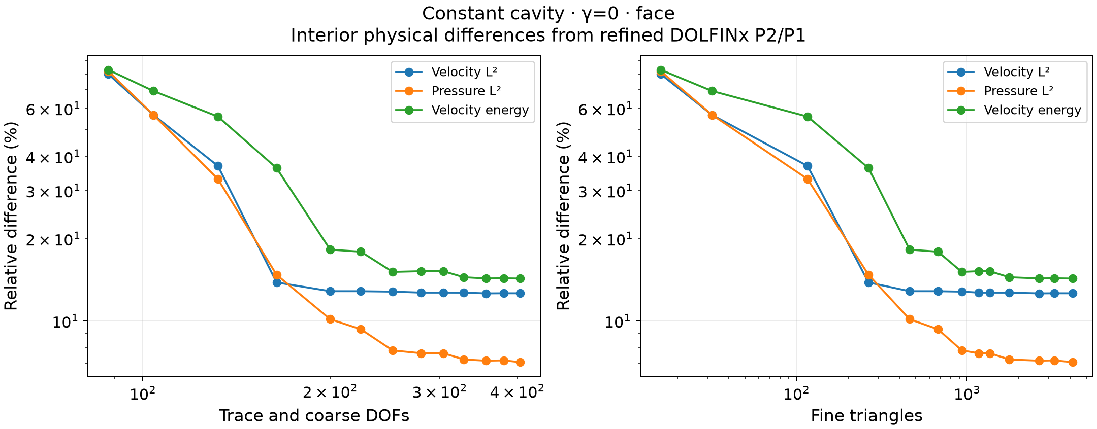
A second face/local configuration uses \(\theta=0.1\) for 21 solved states. It reaches 520 global unknowns and 26,552 fine triangles on the same 16 macrotriangles, retaining a minimum angle of 45 degrees. Its interior differences are 5.010% in velocity L2, 3.723% in pressure L2 and 6.979% in velocity energy. The global velocity L2 difference is 5.003%; pressure and gradient comparisons remain restricted to the interior domain. Changing the final norm quadrature from order 20 to 28 changes the relative energy difference by 0.000054 percentage point. The different maximum-marking threshold and the local resolution are explicit parts of this configuration; the two sequences are not interchangeable accuracy claims based only on global unknown counts.
For macro adaptation, conforming longest-edge closure retains a minimum angle of 45 degrees in the recorded constant-lid series. With \(\theta=0.1\), the Stokes configuration reaches 5,776 trace-plus-coarse unknowns and 1,126 macrotriangles. Its final interior differences are 7.103% in velocity L2, 10.482% in pressure L2 and 22.319% in velocity energy. The physical history also reaches a plateau while refinement continues around the two singular corners. Thus a small geometric scale at those corners does not establish that the remaining interior field is resolved.
For constant-lid Brinkman flow, the macro sequence reaches 19,382 global unknowns and 3,798 macrotriangles. Relative interior differences are 9.407% in velocity L2, 33.966% in pressure L2 and 12.214% in velocity energy. The final four refinement steps leave these interior quantities essentially unchanged while resolving smaller corner scales. The result documents the behavior of the stated maximum-marking rule for singular data; it does not establish that the interior pressure is accurately resolved.
The Brinkman face/local strategy with \(\theta=0.5\) contains 25 solved states. Its final 664 global unknowns and 11,246 fine triangles give interior differences of 5.008% in velocity L2, 9.177% in pressure L2 and 5.034% in velocity energy. The order-20 to order-28 energy comparison changes by 0.000028 percentage point. The physical history records the substantial reduction after local and trace refinement, including its nonmonotone intermediate steps; it is distinct from a claim that the global indicator contracts for discontinuous lid data.
Reproducible numerical records
examples/solve_stokes_adaptive.py writes digested field archives, actual
macro meshes, both estimator components, mixed errors and physical L2 norms.
The uniform and adaptive campaigns run separately from CI:
pixi run --locked -e test-core python -m examples.solve_stokes_adaptive \
  --strategy uniform --viscosity 0.01 --trace-degree 1
pixi run --locked -e test-core python -m examples.solve_stokes_adaptive \
  --strategy macro --viscosity 0.01 --iterations 4
pixi run --locked -e test-core python -m examples.solve_stokes_adaptive \
  --strategy face --viscosity 0.01 --trace-degree 1 --iterations 4
pixi run --locked -e fem python -m examples.solve_cavity_reference --levels 8 16 32 64 128 256 512
pixi run --locked -e notebooks python -m examples.compare_stokes_cavity
pixi run --locked -e notebooks python -m examples.plot_stokes_adaptive
The regression suite checks the element and face formulas independently, including sums outside square roots, ties, zero indicators, inherited local resolution and actual solves. These tests establish discrete contracts; adaptive contraction and optimality are not inferred from them.
References
-
Rodolfo Araya, Ramiro Rebolledo, and Frédéric Valentin (2021). On a multiscale a posteriori error estimator for the Stokes and Brinkman equations, IMA Journal of Numerical Analysis 41(1), 344–380. DOI: 10.1093/imanum/drz053. An earlier version is HAL: hal-01945934v1.
-
Ricardo G. Durán, Lucia Gastaldi, and Ariel L. Lombardi (2019). Analysis of finite element approximations of Stokes equations with non-smooth data. arXiv preprint, version 1, 10 December 2019. arXiv: 1912.04962v1.