Mixed elasticity and near incompressibility

solve_elasticity uses the displacement–Herrmann-pressure formulation. Native GaLS supports P1/P1, P2/P2 and P3/P3 local fields; Taylor–Hood supports P2/P1 and P3/P2. Each macrotriangle retains two translations and one rotation. The displacement-only P1 formulation is selected with formulation="primal".

These native pyMHM experiments compare against exact fields, using bounded forces as the first Lamé modulus grows. The analytical family agrees with the MSL GaLS elasticity case. The curves below are not an independent execution of MSL or a digitized reproduction of the article's figures. The separate MSL GaLS field comparison reports matched runs of both implementations, including higher-order local spaces.

Formulation and constraints

For constant shear modulus \(\mu>0\) and first Lamé modulus \(\lambda>0\),

\[ \sigma=2\mu\varepsilon(u)-pI,\qquad -\nabla\cdot\sigma=f,\qquad \nabla\cdot u+\lambda^{-1}p=0. \]

Thus \(p=-\lambda\nabla\cdot u\). With lame_lambda=np.inf, the pressure compliance is zero. The discrete divergence equation is weak; it does not imply pointwise zero divergence. compressibility_l2() measures \(\|\nabla\cdot u_h+p_h/\lambda\|_0\) directly.

The GaLS residual is \(R(u,p)=2\mu\nabla\cdot\varepsilon(u)-\nabla p\). Stabilization adds \(-\sum_T\alpha h_T^2(R(u,p),R(v,q))_T\) to the bilinear form and \(+\sum_T\alpha h_T^2(f,R(v,q))_T\) to the load. The default \(\alpha\) is half the admissible bound computed from the finite-element inverse inequality, without using an exact solution or a reference error. stabilization_alpha can prescribe another coefficient strictly inside that bound. Taylor–Hood has no GaLS stabilization.

Local stability also requires a compatible traction space. With a linear trace on each segment, GaLS requires at least four fine intervals per segment for P1/P1, two for P2/P2, and one for P3/P3. Segment endpoints must align with the fine boundary mesh. The sufficient degree/refinement conditions follow Lemma 4.5 of the Gomes, Pereira and Valentin (2024, preprint v1). Insufficient pairs are rejected before solving; enriching only the trace does not guarantee stability.

The multiplier is negative Cauchy traction, \(-\sigma n\), while neumann accepts physical outward traction \(\sigma n\) on selected boundary faces. For a fully prescribed displacement boundary, finite compressibility fixes

\[ \int_\Omega p=-\lambda\int_{\partial\Omega}g\cdot n. \]

At infinite \(\lambda\), boundary volume flux must vanish and mean_pressure sets one global pressure gauge. A pure traction problem uses three prescribed rigid_moments; an unbalanced force or moment is rejected. There are no independent pressure gauges on macrocells.

Exact family and printed benchmark conventions

Write \(s=\sin(\pi x)\sin(\pi y)\), \(c=\cos(\pi(x+y))\) and \(\beta=\mu/(\lambda+\mu)=1-2\nu\). On the unit square, let

\[ u_0=\begin{pmatrix} (\cos(2\pi x)-1)\sin(2\pi y)\\ (1-\cos(2\pi y))\sin(2\pi x) \end{pmatrix},\qquad u=u_0+\beta s\begin{pmatrix}1\\1\end{pmatrix}, \]

\[ p=-\mu(1-\beta)\pi\sin(\pi(x+y)), \]

\[ f=4\mu\pi^2\begin{pmatrix} (2\cos(2\pi x)-1)\sin(2\pi y)\\ (1-2\cos(2\pi y))\sin(2\pi x) \end{pmatrix} +\mu\pi^2(2\beta s-c)\begin{pmatrix}1\\1\end{pmatrix}. \]

Displacement vanishes on the boundary and pressure has zero mean. The force stays bounded as \(\beta\to0\), while the limiting pressure remains nonzero. This bounded-load family isolates the effect of the incompressible limit.

The printed §6 data contain a factor mismatch: the displacement correction has amplitude \(\beta/2\), while its pressure uses amplitude \(\beta\); the force also mixes these amplitudes. The equations above use the consistent amplitude-one MSL family. TrigonometricElasticityData(pressure_amplitude=0.5) provides the literal printed displacement with its own consistently derived pressure and force. Independent derivative tests check both choices against \(-\nabla\cdot\sigma=f\).

The additional ElasticityData polynomial family uses a bubble streamfunction and exact integral checks for displacement and elastic energy. Its solenoidal variant has identical displacement and force for every \(\lambda\), providing another independent locking test.

Material sweep

The macro mesh has 32 triangles and one discontinuous linear traction segment per macroface. GaLS P1/P1 uses local refinement 4; GaLS P2/P2 and Taylor–Hood P2/P1 use refinement 2. The two GaLS choices have the same displacement nodal count per macrotriangle. The sweep contains seven paper Poisson ratios, \(\lambda/\mu=10^8\), and the incompressible limit, with \(\mu=1\).

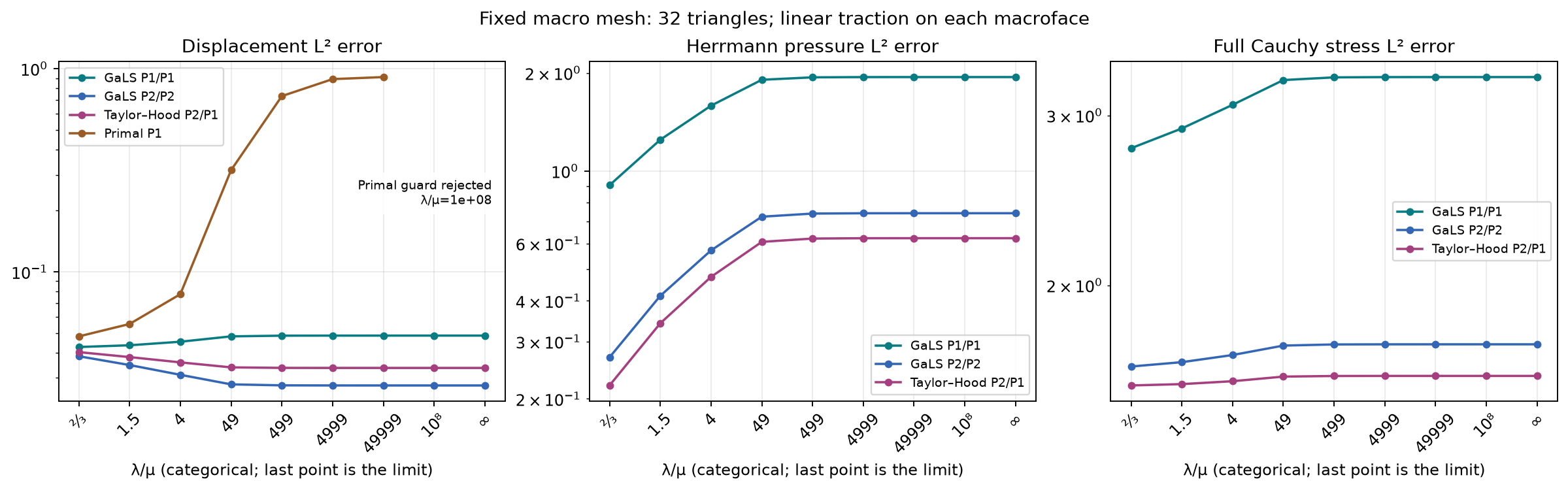
Displacement, pressure and full-stress errors across the material sweep

The horizontal positions are categorical material cases. Slopes on this axis are not convergence rates. Primal points are omitted where the residual or rank checks are not satisfied; the primal formulation does not support infinite \(\lambda\).

Method	u error at ν=0.2	u error at ν=0.4999	u error at λ/μ=10⁸	u error at λ=∞	p error at λ=∞
GaLS P1/P1	4.26018e-02	4.84871e-02	4.84915e-02	4.84915e-02	1.94455e+00
GaLS P2/P2	3.83619e-02	2.75474e-02	2.75440e-02	2.75440e-02	7.42739e-01
Taylor–Hood P2/P1	4.02032e-02	3.36057e-02	3.36035e-02	3.36035e-02	6.22550e-01
Primal P1	4.80492e-02	8.89556e-01	guard rejected	unsupported	unsupported

Here \(\nu=0.4999\) and the same 32 macrotriangles stay fixed. Each macroface has \(s=1,2,3,4,6,8\) traction segments. Local refinement is \(4s\) for P1/P1 and \(2s\) for P2/P2. The maximum segment length is \(H_E=\sqrt{2}/(4s)\). This experiment refines the skeleton and the local spaces together, rather than changing the macro partition. Assembly uses quadrature order 8 and error integration uses order 10.

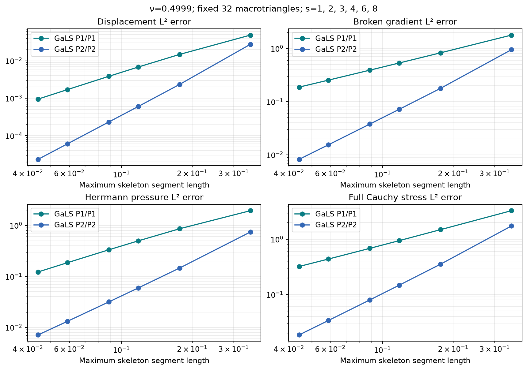
Six measured resolutions for displacement, gradient, pressure and stress

GaLS P1/P1

Segments s	Local refinement	u L²	Broken gradient L²	p L²	Full stress L²	u rate
1	4	4.84871e-02	1.78513e+00	1.94418e+00	3.28867e+00	—
2	8	1.47882e-02	8.29422e-01	8.60290e-01	1.49289e+00	1.713
3	12	6.80138e-03	5.33722e-01	4.97414e-01	9.43204e-01	1.916
4	16	3.84791e-03	3.91327e-01	3.32307e-01	6.83745e-01	1.980
6	24	1.69984e-03	2.54030e-01	1.85750e-01	4.37848e-01	2.015
8	32	9.47632e-04	1.87693e-01	1.22177e-01	3.20943e-01	2.031

GaLS P2/P2

Segments s	Local refinement	u L²	Broken gradient L²	p L²	Full stress L²	u rate
1	2	2.75474e-02	9.48487e-01	7.42557e-01	1.73741e+00	—
2	4	2.33828e-03	1.78339e-01	1.45890e-01	3.53934e-01	3.558
3	6	6.01218e-04	7.18449e-02	5.92959e-02	1.47138e-01	3.350
4	8	2.32281e-04	3.79187e-02	3.15993e-02	7.96268e-02	3.306
6	12	6.05702e-05	1.54700e-02	1.31487e-02	3.37680e-02	3.315
8	16	2.33518e-05	8.23171e-03	7.11226e-03	1.84762e-02	3.313

Rates use \(\log(E_i/E_{i+1})/\log(s_{i+1}/s_i)\) because the segment counts are not all related by a factor of two. They describe this measured sequence, not a universal superconvergence claim.

These observed errors assess the stated spaces and triangulations. They do not certify every heterogeneous material or mesh, and they do not reproduce the article's stabilization coefficients or all its configurations. Stress is the full tensor \(2\mu\varepsilon(u_h)-p_hI\), without substituting a deviatoric or projected quantity.

Fields and one-sided profiles

The displayed case uses P2/P2, \(\nu=0.4999\), two traction segments per macroface and local refinement 4. Exact and numerical panels share a color scale within each quantity. Errors are vector/tensor norms or absolute pressure differences. Every panel shows the actual macrotriangulation.

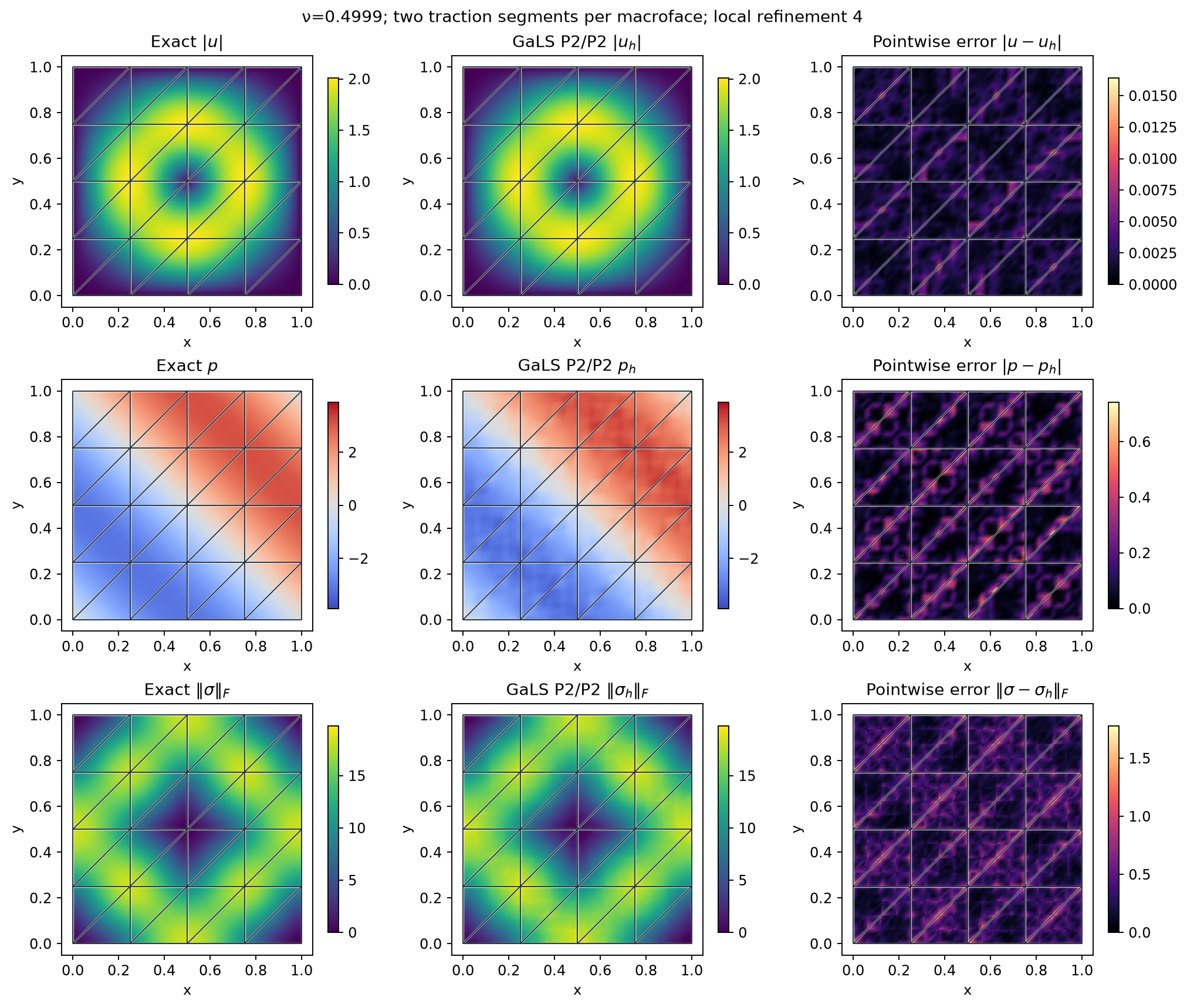
Exact, numerical and pointwise-error maps for displacement, pressure and stress

The spatial-map record identifies the executed case and field digest separately from the original acquisition. Its displacement, pressure, gradient and stress norms agree with the retained configuration to within \(4\times10^{-13}\) relatively.

The profile follows \(y=0.37\). Each macrocell contributes its own endpoint values; opposite traces are neither averaged nor smoothed. Maps sample each finite element separately, whereas norms use physical quadrature directly. This stress field is not an equilibrated H(div) reconstruction. The mixed stress–displacement–rotation method remains a distinct formulation.

Reproduce

The example helpers below are repository sources, supplied separately from the installed library. Open the corresponding notebook to acquire its verified companion, as described in the notebook guide.

import numpy as np
from pymhm import TriangleMesh
from examples.formulations.application import elasticity as solve_elasticity

solution = solve_elasticity(
    TriangleMesh.unit_square(4),
    formulation="gals", degree=1,
    lame_lambda=np.inf, lame_mu=1.0,
    source=(1.0, 0.0), local_refinement=4,
    mean_pressure=0.0,
)

pixi run --locked -e notebooks python -m examples.plot_elasticity --workers 4
pixi run --locked -e notebooks python -m examples.plot_elasticity --reuse-results
pixi run --locked -e notebooks notebooks-run notebooks/elasticity/07_elasticity.ipynb

The first command performs solves and saves JSON, sampled fields and PNG/SVG figures. The second redraws those stored data without PDE solves. Use --workers 1 for serial execution. Worker tests compare assembly, condensation and reconstructed fields between serial, thread and process execution, including a picklable analytical body-force function.

The separate P1 baseline in examples/plot_scalar_elasticity.py uses formulation="primal". It uses \(\lambda=\mu=1\) and five macro meshes; that moderately compressible experiment alone cannot establish resistance to locking. The Methods and bibliography list the original publications for the other elasticity formulations.

References

Antônio Tadeu Azevedo Gomes, Weslley da Silva Pereira, and Frédéric Valentin (2024). A low-order locking-free multiscale finite element method for isotropic elasticity, arXiv preprint, version 1, 25 March 2024. arXiv: 2403.16890v1.